A Kerr black hole, ray-traced in real time
Kerr null geodesics in a WebGL shader: Kerr–Schild, Hamiltonian, three integrators, blackbody Doppler colour. And the fight with the mobile compiler.
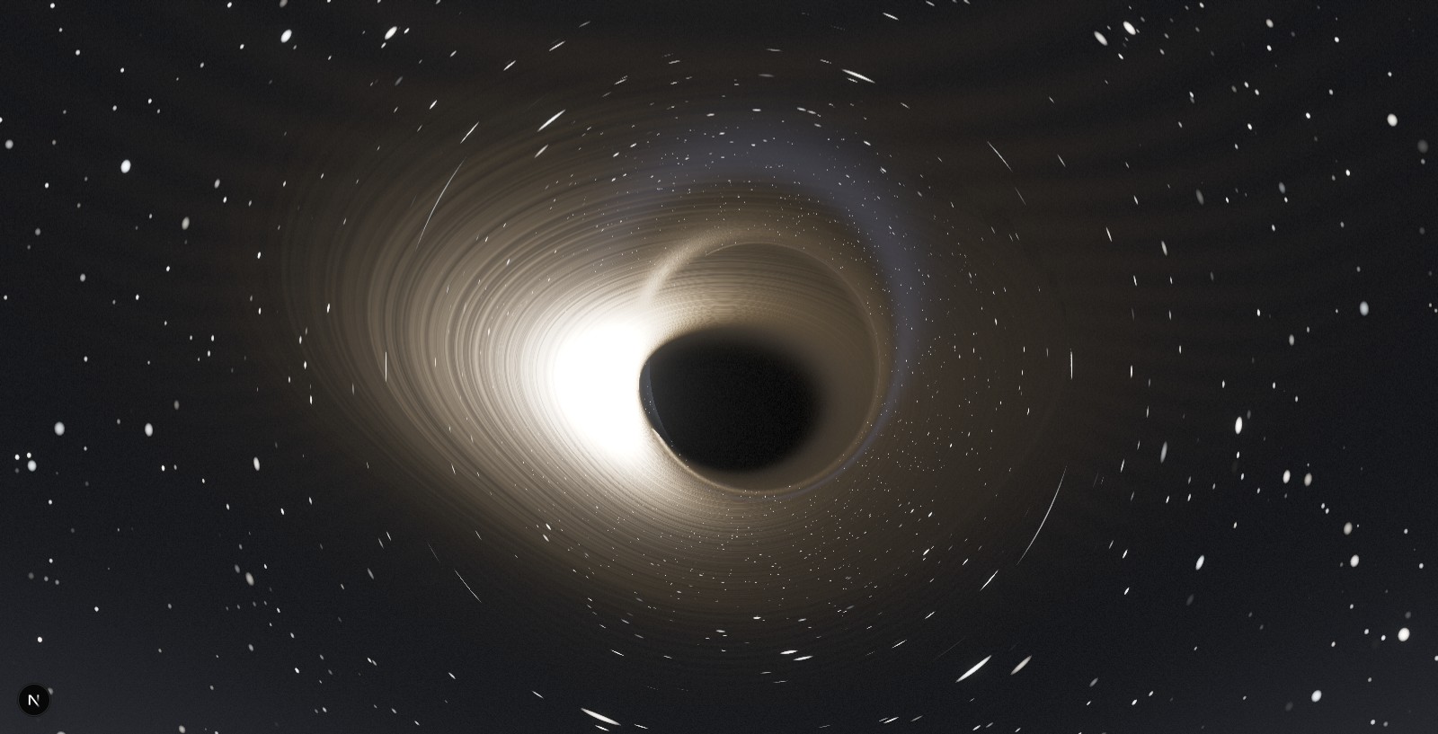
Renderer output: Kerr black hole (spin a = 0.7), lensed accretion disk with Doppler beaming. The approaching side (left) is hotter and brighter. Photon ring: light that orbits 1.5× before reaching the camera. Render: Fosforonero.
The easy part of a black hole simulator is the data. The hard part is running general relativity inside the ~16 milliseconds per frame of a WebGL fragment shader, on a phone. These are the technical notes on how I did it for a Kerr black hole.
The idea: shoot light backwards
For every pixel I shoot a ray from the camera and follow it through curved spacetime. It sounds backwards (light travels toward the eye, not from it), but in general relativity photon paths are reversible: tracing backwards gives the exact same image. That's the trick that spares us from simulating billions of photons that will never hit the screen. We launch one per pixel, exactly the ones we need.
The metric: where the geometry lives
Here gravity is not a force, it's the shape of spacetime, written in the metric . For a rotating black hole I use the Kerr metric in Cartesian Kerr–Schild form:
where is flat Minkowski spacetime, a null vector and the spin. Why this form and not the usual Boyer–Lindquist coordinates? Because it has no coordinate singularity at the horizon and is asymptotically flat: so at the distant camera the photon starts with a trivial momentum (energy , spatial momentum equal to the ray direction) and I never have to build the observer's tetrad, one of the easiest places to get it wrong. At zero spin () it reduces exactly to Schwarzschild.
The integration: Hamiltonian
A photon travels on a null geodesic. I treat it as the flow of a Hamiltonian, because then the step writes cleanly:
The drift (, how the position moves) is closed-form; the kick (, how the momentum changes) I get from finite differences of the gradient of . The step is adaptive: fine near the hole (where curvature matters and the photon ring forms) and coarse far away, after an analytic straight-line advance to the influence sphere, so I don't burn steps in empty space.
Three integrators for three needs
Integrating a differential equation is like walking in the dark in finite steps: too long and you lose the path, too short and you never arrive. I use three "gaits", chosen by quality.
- Symplectic Euler (medium/low): one gradient per step, cheap, 1st order.
- 4th-order Runge–Kutta (high): it samples the slope four times and takes a weighted average,
bringing the deflection error to ~10⁻⁷ rad (verified offline against a reference solution).
- 6th-order Yoshida, symplectic (Ultra): here's a subtlety. Yoshida composes leapfrog steps, but leapfrog wants a separable Hamiltonian; ours isn't. It needs Tao's (2016) method, which doubles the phase space to make it integrable. The «Orbits» demo instead has the Binet equation, which is separable: there a direct Yoshida keeps the energy drift at ~10⁻¹³, shown live.
I don't choose the colour
The disk radiates as a blackbody: each ring has a temperature, from which I get the true Planckian colour. Then I shift it with the relativistic Doppler factor, exact for a Kerr circular orbit:
with the gas angular velocity, the time component of its 4-velocity (the time dilation) and the photon's conserved axial angular momentum. The elegant part: I don't have to "carry" the colour along the ray. The quantity is an invariant (Liouville's theorem: photons neither bunch up nor thin out in phase space), so a blackbody seen with factor stays a blackbody at temperature . No arbitrary palettes, and one side of the disk turns blinding and blue, the other dim and red.
The fight with the mobile shader compiler
The most instructive bug. I had put the Yoshida-6 (Tao) integrator inside the shader. On desktop: perfect. On mobile: the disk disappeared, even at medium quality. The cause wasn't speed, it was size: that code was compiled into the single shader, always, and exceeded the phone GPU's compile budget → the whole full-screen quad failed (lensing and disk together). The fix: gate it behind a GLSL #define, compiled only when you pick "Ultra". The default shader stays small and runs everywhere. The lesson I keep: on mobile WebGL it's how big the program is to compile, not just how fast it runs.
Stack and honesty
Three.js + React Three Fiber, GLSL3, a 16-bit pipeline with anti-banding dithering, KaTeX for the equations. Every approximation is declared: the disk is a model (not a GRMHD solution), the jets are stylized, the playground bodies are not lensed. The full derivation, with academic sources, is on the equations page.
In short: what I take away
- The physics is computable, the emission isn't. Kerr lensing runs in real time; the disk's magnetized plasma (GRMHD) doesn't → you model it and declare it.
- Kerr–Schild avoids the tetrad. At the distant camera the photon's momentum is simply the ray direction: one classic place to slip, removed.
- You don't choose the colour. The invariant Iᵥ/ν³ (Liouville) carries a blackbody from T to g·T without transporting anything along the ray.
- On mobile WebGL it's the shader's size that bites, not just its speed. The Ultra integrator lives behind a
#define, compiled only when needed, otherwise the whole quad failed on phones.