Black hole: a mathematical and physical treatment

Abstract

We describe a real-time WebGL renderer of a Schwarzschild black hole and its accretion disk. For each pixel we cast a ray from the camera backwards and integrate the photon's exact null geodesic through curved spacetime, the same path a real photon follows, by numerically solving the equations of general relativity (backward tracing gives the same image because light paths in GR are reversible): a true simulation of the lensing, not a graphical effect. This yields gravitational lensing, the photon sphere, the shadow and, through returning radiation, the photon ring. The disk is optically thick with blackbody emission and invariant relativistic radiative transfer (g⁴ beaming, gravitational redshift). A companion demo integrates the exact timelike geodesics (periastron precession, ISCO), while a playground uses the Paczyński–Wiita pseudo-Newtonian potential for N-body dynamics with tidal disruption. The approximations are stated explicitly: spin is now the exact Kerr metric (null geodesics ray-traced in real time), and the disk follows it too (inner edge at the prograde ISCO, exact Kerr Doppler and redshift, and a relativistic thin-disk (Shakura–Sunyaev) radial flux with the Kerr-ISCO inner edge, while the exact Page–Thorne integral is shown in the equations as the relativistic reference); the turbulence is procedural (not GRMHD), and the jets are stylized.

1. Schwarzschild metric and null geodesics

Start with the stage. Around a non-rotating spherical mass, empty spacetime can take only one shape, the Schwarzschild solution, found in 1916. It is how the mass tells space and time to curve. Two symmetries hand us two gifts: because the geometry changes neither in time nor under rotation about the axis, there are two quantities a photon keeps for its entire journey, an energy E and an angular momentum L. They are our fixed points in a world that bends.

Now add light. A photon is massless and travels on a null geodesic: its spacetime «length» is exactly zero. Confine it to the equatorial plane and the whole problem collapses into something surprisingly familiar, a ball rolling in a valley, with an effective potential. The classic trick is to change variable, u = 1/r: the orbit becomes the Binet equation. Compared with Newton there is just one extra term, that 3M u², and it is all of general relativity packed into three symbols: negligible far away, the master up close.

That term does something spectacular: at r = 3M light itself can settle into a circular orbit. This is the photon sphere, an orbit so unstable that the faintest nudge throws the photon in or sets it free. And it is the edge of the shadow.

It's worth watching it appear, not just stating it (the equation is below). From the effective potential a photon turns back where its radial velocity vanishes, which ties its impact parameter to the radius of closest approach: 1/b² = (1/r²)(1 − 2M/r). The «critical» photon is the one that skims on the edge, and it sits at the maximum of that curve. Differentiating and setting it to zero, d/dr[1/r² − 2M/r³] = −2/r³ + 6M/r⁴ = 0, gives r = 3M: the photon sphere falls out of the calculation, we don't put it in by hand. Substituting r = 3M back into the impact-parameter formula gives the shadow's exact threshold: 1/b_c² = (1 − 2/3)/(9M²) = 1/(27M²), i.e. b_c = 3√3·M ≈ 2.6 rₛ.

Translated into what a distant eye sees: every ray with impact parameter b = L/E below this b_c is doomed to fall, while those just above wind around the photon sphere and come back, and it is from that returning light that the thin bright ring is born. The renderer does nothing but integrate this trajectory, ray by ray (symplectic Euler, or 4th-order Runge–Kutta on High quality). (Carroll, Caltech; Kokkotas, Univ. Tübingen; Hirata, Ohio State; MTW.)

2. Timelike geodesics: orbits, ISCO, precession

Swap the photon for a stone. Now the «length» of the path is not zero but −1, the ticking of its own clock, and the same pattern returns: a ball in an effective potential V_eff. But the valley has a new shape. In Newton there is always a dip where a stable orbit can sit, however tight; in Schwarzschild that dip vanishes if you get too close. The point of no return is r = 6M = 3 rₛ, the ISCO, the innermost stable circular orbit: one step further in and no orbit holds, the stone slides in with no appeal. This has no Newtonian analogue; it is the signature of the strong field.

Where does that 6M come from? It's worth deriving (the equations are below). A circular orbit lives at a stationary point of the potential, dV_eff²/dr = 0: this fixes the angular momentum required at that radius, L²_circ = M r²/(r − 3M). Notice it diverges at r = 3M, the photon limit, the innermost circular orbit possible at all. But «possible» isn't «stable»: a stable orbit sits at the bottom of a dip, so it also wants d²V_eff²/dr² > 0. The two demands collide as you approach the hole and meet, the dip flattening into an inflection, exactly at r = 6M. That is the ISCO: a hair further in the dip is gone, and nothing holds the stone.

And the orbits that do not plunge? They do not close. The very 3M u² that ruled the light here slowly rotates the ellipse on every turn: the periastron advances and the orbit traces a rosette. It is, literally, the mathematics of the famous 43 arc-seconds per century «too many» in Mercury's precession, the anomaly that in 1915 gave Einstein his first observational confirmation. In the weak field the advance per orbit is Δφ ≈ 6πM/p (with p the semi-latus rectum): tiny for Mercury, enormous near the hole. In the «Orbits» demo, just push L below the 2√3·M threshold to watch the rosette turn into a plunge.

A geometric note: by spherical symmetry every Schwarzschild orbit lies in a fixed plane. The «Inclination» slider orients that plane in space (the integration stays exact), so the orbit is genuinely seen in 3D relative to the equatorial disk. Truly non-planar orbits, the ones that fill a spherical shell, exist only around a rotating (Kerr) hole and are governed by a fourth conserved quantity, the Carter constant. In plain terms: to integrate an orbit you need as many «conservation laws» as the motion has dimensions. Schwarzschild's spherical symmetry already hands you enough (energy, angular momentum); Kerr, symmetric only about its axis, would lose one, but Carter found in 1968 that a fourth, hidden one survives, and it is what makes the equations solvable again instead of chaotic.

3. Relativistic accretion disk

The disk is gas spiralling toward the hole, and as it falls friction and turbulence heat it until it glows. The classic model is Shakura & Sunyaev's (1973), later cast in relativistic form by Novikov & Thorne, with one elegant boundary condition: at the ISCO the stress vanishes, because there the gas loses its grip and plunges. From how much energy each ring radiates follows, via Stefan–Boltzmann, its temperature, rising toward the centre as r⁻³ᐟ⁴. The renderer uses this thin-disk profile in analytic form, with the inner edge pinned to the Kerr ISCO; the exact orbit-averaged Page–Thorne integral is the one in the equations below, the relativistic reference the profile descends from.

But what is actually missing? A real disk is not a smooth radiating surface: it is plasma (ionised gas) threaded with magnetic fields, and what drives it toward the hole is a very specific turbulence. This is where the acronym I keep using without unpacking comes in: GRMHD, «general-relativistic magnetohydrodynamics». It means solving together, on the grid of curved spacetime, the equations of the fluid and those of the magnetic field (Maxwell). You need it because in disks it is the magnetorotational instability, the MRI (an instability of magnetised, differentially-rotating plasma that Balbus & Hawley showed applies to disks in 1991), that carries angular momentum outward and lets the gas fall in. Without magnetic fields a disk would not even know how to accrete. A GRMHD simulation computes all of it: the real turbulence, the synchrotron emission of electrons spiralling in the fields, full radiative transfer. It is the state of the art (the codes are called HARM, Athena++, BHAC, KORAL) and it is what made the Event Horizon Telescope images interpretable. But it costs minutes to hours per single frame, on a supercomputer. Inside the ~16 ms of a browser shader there is no hope. That is why our gaseous structure is procedural turbulence: it mimics the look, not the physics. The thermal side (temperature, colour, redshift, beaming) is the real thing.

And here is the part we like best: we do not choose the colour. Every point on the disk has a temperature, and that temperature has a true blackbody colour, the same as a poker glowing red, then orange, then blue-white as it heats. We convert that temperature to its colour along the Planckian locus and show it, with no arbitrary gradient. The first to compute the image of such a disk, by hand, in 1979, was Jean-Pierre Luminet, and it already looked like Interstellar. (Shakura–Sunyaev 1973; Novikov–Thorne 1973; Luminet 1979.)

A word on the edges, because they tell two opposite stories. The inner one is genuinely sharp: at the ISCO the gas departs and the light simply ends there. The outer one is not: it depends on where the disk is fed, and it is fuzzy. In reality the brightness already falls on its own as r⁻³; we add a soft, wide taper that dies out with vanishing slope, so the rim is not cut with a knife. The disk is also rendered as an optical-depth medium: opaque where bright (inner), translucent where faint (outer), with each plane crossing's opacity ∝ brightness/|cosθ|, so edge-on (a long path through the gas) it reads as dense, face-on as thin, with no geometric slab and no black seam.

4. Radiative transfer and relativistic effects

How does the light change along the way? There is an almost magical quantity that stays constant: the intensity divided by the frequency cubed, Iᵥ/ν³. It is Liouville's theorem in disguise: photons, in their phase space, neither crowd together nor thin out. If we know it where the light is born, we know it here at the eye. All the work then boils down to one number: the factor g, the ratio of the frequency we receive to the one emitted.

That g rolls three effects into one: time running slower near the mass (gravitational redshift), the time dilation of the racing gas, and the Doppler of whatever comes toward us or flees. A blackbody seen with factor g stays a blackbody, but at temperature g·T, so g shifts colour and brightness together. The result is an unmistakable signature: the side coming at us is dazzling and bluish, the side fleeing dim and red. And since brightness goes as g⁴, it takes little for one side to dominate the other. (Luminet 1979; Vincent et al. 2011, GYOTO.)

But why the fourth power, and not the first or the second? It's worth taking apart, because it's one of those counts where three different things conspire to the same exponent. Picture the photons as a rain you are counting. (1) Each drop that arrives carries energy hν, and the frequency is already shifted by g: one factor of g. (2) More of them arrive per second, because the rate of arrivals is dilated by the same g (an approaching source's clock «ticks» faster for us): a second factor of g. (3) And the beam the source emits wide is squeezed forward by relativistic aberration (whoever rushes toward us concentrates their light into a narrower cone), so the solid angle contracts as g²: two more factors. One times one times two: g⁴. It is also why the natural invariant is not the intensity Iᵥ but Iᵥ/ν³: that ν³ is exactly the «energy × rate × solid angle» product that drags the factor g along, so dividing it out leaves a number the journey no longer touches. The renderer works precisely this way: it carries Iᵥ/ν³ from the disk to the eye unchanged, and only at the end multiplies by the g⁴ of the emission point.

5. Returning radiation and the photon ring

Here is what makes a black hole so luminous. Some rays go neither straight nor in: they graze the photon sphere, make half a turn, a turn, two turns around the hole, and then leave. This is returning radiation: the disk's own light coming back into view after passing behind the horizon. To catch it the renderer refines its steps exactly where the path winds, where a coarse step would miss the loop.

The result is a ladder of ever-thinner images of the disk, stacked side by side, crowding toward the edge of the shadow. Each extra turn shrinks the image by a fixed factor, exponentially, with Lyapunov exponent γ = π for Schwarzschild, until they merge into the bright thread of the photon ring. The part we are proud of: we do not draw it. It emerges on its own from the real returning disk light, in the same colour, with no fake ring laid on top. (Luminet 1979; Gralla, Holz & Wald 2019; Johnson et al. 2020, EHT.)

How fast do these rings close in? There's a clean number behind it, and it makes sense once you think about what «unstable orbit» means. A ray grazing the photon sphere is like a pencil balanced on its tip: the slightest deviation grows, and grows exponentially. The rate of that growth is the orbit's Lyapunov exponent, and for Schwarzschild it is exactly γ = π. Turned around, it says: to make one more loop around the hole before escaping, a ray must start closer to the critical value b_c by a factor e^{−π} ≈ 1/23. So each successive image of the disk is ~23 times thinner and ~23 times fainter than the last. It is a merciless geometric ladder: the first ring you see, the second barely, the third is already below any practical threshold. That is why «the» photon ring, in the real images, is effectively a single one: the others are there, crushed against the edge of the shadow. We don't draw them, we let them emerge by refining the integrator's steps exactly where the path winds.

The same mechanism inscribes its signature on the background star field, not just the disk. Every background star in fact has infinitely many distinct images: the primary (rays that never orbit), the secondary (rays that orbit once), the tertiary, and so on. The boundary between successive orders is a genuine mathematical caustic — a ray just outside does not orbit, a ray just inside orbits exactly once — and produces sharp circular rings in the star field, nested around the shadow with a spacing that shrinks by e^{−π} ≈ 1/23 per order. These rings are not a graphical artifact: they appear in every correct GR ray tracer, including the DNGR code that produced Gargantua for Interstellar (James et al. 2015). If you see them in the render, it means the integrator is correctly resolving the caustic structure of the lensing.

6. Rotation: Kerr and frame dragging

Real black holes spin, and a spinning black hole does something astonishing: it drags space itself around with it, the way a whirlpool drags water. Close enough you cannot stay still even at full thrust: space carries you along. The correct metric is Kerr's, and that dragging (frame-dragging) has a precise angular velocity ω = −g_{tφ}/g_{φφ}.

Where does that ω come from? Imagine dropping something «straight down», with zero angular momentum. In Kerr it doesn't fall straight: it gets dragged into rotation, and its angular velocity is exactly ω = −g_{tφ}/g_{φφ}, the direct consequence of the off-diagonal g_{tφ} term that rotation adds to the metric. Far away it fades as 1/r³ (the Lense–Thirring effect, the same one measured around the Earth by Gravity Probe B); close in it becomes irresistible. So much so that inside a surface called the ergosphere, no one can stay still relative to the distant stars: to do so they'd have to exceed the speed of light. It's the region where the g_{tt} component changes sign; its boundary at the equator reaches r = 2M, outside the horizon. There, space flows faster than anyone could swim against it.

And here the renderer goes all in: with the Spin slider we integrate the EXACT Kerr null geodesics, in Cartesian Kerr–Schild form. That form has no Boyer–Lindquist coordinate singularity and is asymptotically flat, so the photon's initial momentum at the (distant) camera is simply the ray direction, with no observer tetrad to get wrong. A tetrad is the observer's local orthonormal frame (their four «rulers and clock»): in awkward coordinates you must build it by hand to turn what the camera measures into what the metric calls momentum, and it's a classic place to slip. Here, asymptotically flat, that translation is the identity. The asymmetric shadow, the displaced and flattened photon ring and the dragging of inertial frames all emerge on their own: the same physics as Interstellar's Gargantua (James, von Tunzelmann, Franklin & Thorne 2015), there ray-traced offline, here in real time in the browser. The disk now follows Kerr too: the inner edge sits at the prograde ISCO (Bardeen) and the Doppler/redshift come from the exact Kerr metric (g = 1/[uᵗ(1−Ωλ)] with λ the photon's conserved axial angular momentum), and the radial flux is the relativistic thin-disk (Shakura–Sunyaev) profile with that Kerr-ISCO inner edge, so the hot region tightens toward the smaller ISCO as the hole spins up. (Bardeen 1972/1973 for the ISCO and Kerr geodesics; the exact Page–Thorne 1974 flux is shown in the equations as the relativistic reference.) The latest data back this choice: a Bayesian neural-network analysis of the EHT data (Janssen et al. 2025) points to a near-maximal spin (a ≈ 0.8–0.9) and a near face-on disk for Sgr A*, exactly the regime where these Kerr effects are most pronounced.

7. Spatial geometry: Flamm's paraboloid

The rubber sheet with the bowling ball is a beautiful image and almost always wrong. The grid you can switch on, instead, is the right one: Flamm's paraboloid (1916). Take the equatorial slice of the space around the hole (t, θ = π/2 const) and embed it, without stretching, into ordinary 3D Euclidean space, and you get exactly that funnel. Distances measured on the surface are the true distances of Schwarzschild's curved space: not a metaphor but its intrinsic geometry drawn faithfully. When the hole spins, the funnel twists: that is frame-dragging made visible.

Where does that funnel shape come from? It derives in three lines, and they are three lines worth following. Freeze time and stand in the equatorial plane: the true distance between two nearby points, in Schwarzschild's space, is dℓ² = (1−rₛ/r)⁻¹ dr² + r² dφ². That (1−rₛ/r)⁻¹ in front of dr² is the whole point: it says that to move one «coordinate metre» radially, near the hole, you must cross MORE than one metre of actual space. Now ask which surface of revolution z(r), in ordinary Euclidean space, would have those same distances: on such a surface dℓ² = (1+(dz/dr)²) dr² + r² dφ². For the two to agree just match the dr² coefficients, and out comes (dz/dr)² = (1−rₛ/r)⁻¹ − 1. Integrating gives z(r) = 2√(rₛ(r−rₛ)). The funnel isn't chosen for resemblance: it is the only surface that reproduces, without cheating, the intrinsic geometry of that slice of space.

A warning, though, because this is where the «rubber sheet» really misleads. This funnel is a slice of space ALONE, photographed at one instant: it contains no time. And in relativity things fall mainly because they are deflected in curved TIME, not because they «roll downhill» along a spatial slope. The ball on the sheet, after all, accelerates because of the Earth's gravity pulling down, beneath the sheet: that's circular reasoning, explaining gravity with gravity. Flamm's funnel makes no such error: it does not explain why you fall, it only measures how much extra space there is to cross as you approach the hole. The actual falling is computed by the geodesics, which live in the full spacetime, and that is exactly what the renderer integrates.

8. Playground: body dynamics

The playground trades a little exactness for the fun of throwing things in and watching. Instead of the full geodesics it uses a famous trick: the Paczyński–Wiita potential, Φ = −GM/(r − rₛ). It looks like Newton, but that −rₛ in the denominator works the magic: it reproduces the ISCO at 6M and the final plunge exactly, the strong-field effects Newton lacks. In return we can afford real mutual gravity between all the bodies (a softened N-body). The «System» button builds, in one go, a small inclined planetary system with the black hole standing in for the central star, like Gargantua.

And when a body comes too close? It gets spaghettified. The tide, the difference in gravity between the body's near and far sides, overcomes its self-grip and stretches it. The key physics (Rees 1988) is a spread in energy: half the debris slows and falls back, wrapping around the hole and feeding the disk; the other half speeds up and is flung out in a long tail. The fallback follows the famous Ṁ ∝ t⁻⁵ᐟ³ law. Even before full disruption the star sheds gas from the cap facing the hole, a veil that widens as it sinks. (Paczyński–Wiita 1980; Rees 1988.)

Where does that −5/3 come from, the exponent that signs every tidal disruption ever observed? It is surprisingly elementary: it is just Kepler. At the instant the star is stretched, each piece of it ends up with a slightly different energy (whatever was on the near side loses energy, whatever was on the far side gains it), and this range of energies ε is, to first approximation, uniformly spread. Each bound piece (ε < 0) returns on an ellipse, and Kepler's third law ties its period to its energy: T ∝ |ε|⁻³ᐟ². So the debris returns in order: first the most bound (large |ε|, short period), then the lazier ones in turn. The rate at which mass falls back is Ṁ = (dM/dε)·(dε/dt): the first factor is nearly constant (the spread is flat), and the second you get by inverting Kepler: from T ∝ |ε|⁻³ᐟ² and t = T it follows that ε ∝ t⁻²ᐟ³, hence dε/dt ∝ t⁻⁵ᐟ³. There is the −5/3: not a number handed down from above, but the signature of Kepler's third law applied to a cloud of debris coming home in order of energy. (Rees 1988.)

Two bodies that touch do not pass through each other: they merge, conserving mass and momentum (the radius combines by volume). And the «GW» button switches on radiation reaction: bodies emit gravitational waves, lose energy and spiral toward the hole, a miniature EMRI, the fall accelerating headlong (the «chirp») because the radiated power grows as 1/r⁵, down to the plunge or merger. The real effect is minuscule, ∝ (v/c)⁵: here it is amplified to be visible, exactly like the time speed-up. (Peters 1964.)

In WebGPU mode the Playground runs 300,000 particles on exact prograde Kerr orbits with small epicyclic perturbations (radial epicyclic frequency κ, the same that vanishes at the ISCO): the accretion disk is live, not a painted image. The «Ringdown» button simulates a perturbation: the photon ring (the returning radiation — rays that have made at least one loop around the hole) pulses with the damped sinusoid A(t) = exp(−ω_I·t)·cos(ω_R·t), calibrated to tabulated Kerr l=2 quasi-normal mode frequencies (Leaver 1985). The quality factor Q = ω_R/(2ω_I) = 2.1 + 11.3·a³ is physically correct: at zero spin the hole rings ~2 times; near a≈0.99 it rings ~13 times before settling — the same signature LIGO measures in the tail of every black-hole merger. Vary the spin and watch the decay change.

9. Numerical methods of the renderer

Lensing: we integrate the EXACT Kerr null geodesics in Kerr–Schild Hamiltonian form (the drift dx/dλ = ∂H/∂p is closed-form, the kick dp/dλ = −½∇ₓHq is by central finite differences), with an adaptive step refined near the photon sphere for the returning radiation. Two integrators selected by quality: symplectic Euler (1st order, one gradient per step) for Medium/Low, and 4th-order Runge–Kutta for High. RK4 brings the deflection error to ~10⁻⁷ rad and keeps the null invariant Hq constant to ~10⁻⁶ (verified offline against a reference solution), at the cost of four gradient evaluations per step. Tone mapping is ACES filmic followed by gamma correction.

Playground: dynamics in the Paczyński–Wiita potential use adaptive sub-stepping with softened mutual gravity (softening ε) and speeds capped at c. The step, however, is stability-limited: it never exceeds a fraction of the local dynamical time near the hole (a CFL-like criterion, h ≤ min(h_max, C·(r−rₛ))). If the sub-step budget is not enough close to the horizon, the simulation advances less simulated time (it gently slows down) instead of stretching the step and injecting energy, so the N-body system stays stable even with many bodies. The semi-implicit (symplectic) update conserves energy, so bound orbits stay bound and moons orbit with the circular speed of the same softened force the integrator uses (they do not unbind). Tidal debris lives in a fixed-size pool (ring buffer). The «Orbits» demo integrates the exact timelike orbit equation in the azimuth φ.

How trustworthy is the integration? The «Orbits» demo shows, live, the drift of the orbit's energy invariant C (the first integral of the equation, tied to E): with the 6th-order Yoshida symplectic step it stays around 10⁻¹³ and oscillating rather than growing: the numerical proof that energy is not leaking and that bound orbits stay bound. (Leapfrog/Yoshida needs a separable Hamiltonian like this one; for the lensing, whose Hamiltonian is non-separable, we use RK4 instead.)

10. Ray-marching robustness and artifacts resolved

The per-ray step budget is finite: to avoid spending it just reaching the hole (which made the disk and shadow glitch when zooming far out), rays starting beyond the influence sphere R_far are advanced analytically in a straight line (spacetime there is essentially flat) and the geodesic march only begins where curvature matters. That is why the view holds even at large distance. Rays that never enter the influence sphere do not sample a «straight» sky, though: they receive Einstein's analytic weak-field deflection — the angle α = 4M/b, weighted for the camera-to-infinity stretch only — so the lensing decays smoothly with growing impact parameter instead of switching off at the sphere's rim, which otherwise showed in the sky as a large circular seam. Near the photon sphere, by contrast, the step is refined to resolve returning radiation and the sub-rings; and inside the 3D volumetric disk's thickness the step is bound to the local scale height H(r), in proportion to the ray's vertical slope, so the hydrostatic Gaussian is sampled densely enough not to render as discrete slabs (banding) — while plane-skimming rays, which see no vertical variation, keep the long step and never exhaust the budget.

Depth compositing: the lensed hole writes depth (gl_FragDepth) from the world-space hit point, so the 3D bodies, particles and playground debris are correctly occluded by the disk and horizon instead of drawing on top. Tone mapping is ACES filmic with a high-threshold bloom, and the sky background has a near-zero floor: deep space stays black (Olbers' paradox), as it should.

Disk aliasing: the turbulence is not a tiled texture (which left a grid-like «checkering» and a seam line) but a gradient-noise (Perlin) FBM with a lattice rotated at each octave and a domain warp, so neither a checkerboard nor lattice facets appear. To remove grazing-angle perspective shimmer, each octave is also band-limited (filtered FBM, mip-style): its frequency is compared with the pixel's footprint on the disk, estimated analytically from distance and crossing angle (NOT from fwidth of the ray-marched hit point, which varied in 2×2 blocks and produced a screen-aligned «net»), and the octave fades toward its mean once its period drops below one pixel. The photon ring is not drawn analytically (no «double ring»): it emerges from the real disk light via returning radiation. Finally the post-processing runs in a 16-bit (float) pipeline with a final dither, so the disk's smooth gradients show no 8-bit banding.

Optional rendering styles. «Starless» evokes the photographic look of Riccardo Antonelli's raytracer (rantonels/starless) by enriching the procedural sky into a structured, dust-laned Milky Way with denser stars: because it is sampled with the ALREADY-lensed ray direction, the rich sky is genuinely warped by the hole (the starless signature), without shipping a multi-MB panorama. «EHT» renders at very low (beam-limited) resolution to mimic the real Event Horizon Telescope images of M87* and Sgr A*.

11. Limits: what it is NOT (scientific honesty)

Spin is now the exact Kerr metric (null geodesics ray-traced in real time), and the disk follows it for the ISCO and the Doppler/redshift; the radial flux profile is instead a relativistic thin-disk (Shakura–Sunyaev) profile with the Kerr-ISCO inner edge, not the Page–Thorne integral evaluated in real time (we show it in the equations as the reference). The disk is optically thick with blackbody emission: its turbulent gaseous structure is a procedural stand-in for magnetorotational (MRI) turbulence, not a GRMHD solution; it does not model self-gravity, vertical thickness or polarization. The photon ring emerges from returning radiation but the very high-order images are not resolved; the relativistic jets are a stylized (optically-thin) addition, not MHD. Background stars are procedural (their lensing is real). In the playground the bodies are occluded by the disk/horizon but not lensed, the integration is pseudo-Newtonian and the disk lighting is a central light (an approximation).

In short, what is NOT possible in this medium, and why. (i) Kerr lensing (null geodesics) we now do in real time, but a GRMHD disk solution in the Kerr metric (full radiative transfer of the magnetized gas) takes minutes-to-hours per frame on compute clusters: incompatible with the ~16 ms per frame of a WebGL fragment shader. (ii) Very high-order photon-ring images (n ≳ 2) demand a numerical precision and a per-pixel step count the real-time budget cannot afford. (iii) Full radiative transfer (multiple scattering, polarization, frequency-dependent opacity), vertical thickness, self-gravity and the hydrodynamics of the disk and tidal streams are time-dependent 3D problems, out of reach for a single shading pass. (iv) Lensing and GR-integrating every playground body would multiply the cost by the number of bodies, killing interactivity. All of this is done, but offline, with the cited GR codes (GYOTO, RAPTOR, ipole…): which is exactly why they exist.

12. Differences from Interstellar (Gargantua / DNGR)

Gargantua, the black hole in Interstellar (2014), was computed by Double Negative with a dedicated engine, DNGR (Double Negative Gravitational Renderer), described in a genuine scientific paper (James, von Tunzelmann, Franklin & Thorne 2015). The underlying physics is THE SAME we use here: exact Kerr null geodesics. Everything else differs, and it is instructive to see why.

Time and resolution. DNGR ran OFFLINE on a render farm: up to ~hours per frame at IMAX resolution (tens of megapixels), with hundreds of TB of data for some sequences. We compute the same lensing in ~16 ms per frame in the browser. To do that we trace a single ray per pixel; DNGR traced whole BUNDLES of rays and propagated their cross-section, so it could accurately anti-alias and filter the razor-thin features (the photon ring, the disk edges), a luxury we cannot afford at 16 ms and which we replace with supersampling, noise band-limiting and dithering.

The disk. Theirs was a bespoke artistic-volumetric model built by the artists (with textures, thickness, swirls), not a GRMHD simulation; ours is an optically-thick surface with true blackbody emission and a relativistic thin-disk flux, textured with procedural turbulence. Both are models of the gas, not magnetohydrodynamic solutions.

A famous NARRATIVE choice: in the film the disk is almost symmetric in brightness. In reality relativistic beaming makes one side blinding and the other dim (Doppler asymmetry), and Christopher Nolan and Kip Thorne chose to SUPPRESS it because such a lopsided image would confuse the audience. We do the opposite: we show the real Doppler asymmetry (you can toggle it) because the goal here is educational, not cinematic. For the same reason they used a near-extremal spin (a/M ≈ 0.999, for the plot's time dilation); here spin is a slider.

In one line: same metric, same geodesics; theirs offline, photoreal, with artistic licence in service of the story; ours real-time, interactive, with the real physics laid bare and every approximation disclosed.

13. Design choices: why this way

Every decision here springs from a single tension: maximum physical truth within the ~16 ms per frame of a browser fragment shader. Here are the main choices and their reasons.

Compute, don't draw. The lensing is the «wow» and it is exactly computable, so we genuinely integrate it (geodesics), ray by ray. The disk emission, by contrast, is NOT computable in real time (it would need GRMHD), so we use a physically-motivated procedural model and DECLARE it. The «fail loud, never fake» rule runs through the whole project: no invented metrics, no arbitrary colours, every approximation stated in black and white.

Kerr–Schild form (not Boyer–Lindquist). Boyer–Lindquist coordinates have a horizon singularity; Kerr–Schild does not, and is asymptotically flat: so the photon's initial 4-momentum at the distant camera is simply the ray direction (E=1), with no observer tetrad to get wrong and no horizon instability.

The right integrator for each problem. The lensing has a NON-separable Hamiltonian → we use RK4 (4th order, ~10⁻⁷ rad per ray); the orbit demo has the SEPARABLE Binet equation → we use a 6th-order Yoshida symplectic step (energy drift ~10⁻¹³); the playground trades exactness for interactivity with the Paczyński–Wiita pseudo-Newtonian potential, which reproduces ISCO and plunge but allows N-body gravity (lensing and GR-integrating every body would kill interactivity).

Optical-depth disk, not a geometric slab: it removes the black edge and the banding and gives a smooth radial transition. 16-bit pipeline + dithering: no 8-bit terracing on the smooth gradients. Colour from temperature (blackbody), not from a palette. Relativistic thin-disk flux, not an arbitrary gradient. Analytic fast-forward to the influence sphere plus an adaptive step: we spend the step budget where it matters (near the hole), not in empty space.

Adaptive quality, one render per device. The same shader must run on an entry-level phone and on a discrete-GPU workstation, and WebGL has no vendor-specific code (one GLSL for everyone), so the real lever is dosing the load. The «Auto» mode detects the GPU (via WEBGL_debug_renderer_info: NVIDIA/Radeon/Apple-Silicon on desktop, Adreno/Mali/Apple on mobile) and picks a profile: on high-end desktop the Yoshida-6 integrator, 2× supersampling and the volumetric disk; on mobile the cheaper Euler integrator with more steps and a capped DPR, because there the bottleneck is fill-rate, not steps. Since some browsers mask the GPU for privacy, a governor measures the FPS (exponential moving average) and dynamically scales the load: on mobile the render resolution first (the bottleneck is fill-rate), then — only if that is not enough — the step count; on desktop the steps. Resizing the canvas is itself a small hitch, though, so the governor is anti-oscillation: a resolution that dropped the FPS becomes a ceiling it never climbs back to (otherwise vsync, quantising FPS to 60↔30, would bounce it between the two thresholds forever), recovery waits out a cooldown, and the FPS average restarts after every adjustment so the resize hitch does not pollute the next measurement. The heavy modes (Ultra, supersampling, 3D disk) stay isolated behind GLSL #defines compiled only when needed, so the default mobile shader stays small and compiles everywhere.

Three separate modes (lensing, orbits, playground) because they separate different concerns: rigorous single-body GR vs many-body interactivity. A light procedural sky by default, with the «Real sky» option (a lensed NASA equirectangular photo) when you want the true sky. And finally accessibility: bilingual, free, ad-free, usable from a phone: real physics should be within everyone's reach.

The real images: M87* and Sgr A*

Event Horizon Telescope images are not photographs in the ordinary sense: they are radio-interferometry maps at very short wavelength (1.3 mm, 230 GHz), assembled by combining signals from telescopes spread across the planet to simulate an Earth-sized radio dish. The result is an angular resolution of ~20 microarcseconds for M87* and ~25 for Sgr A* — just enough to resolve the shadow.

The orange ring is not a flame: it is the millimetre-wavelength light of hot plasma around the hole, amplified by gravitational lensing. The asymmetric brightness (brighter on the left for M87*, time-variable for Sgr A*) is exactly the Doppler beaming shown in our render. The dark central region corresponds to the b_crit parameter in the Real Scale panel formula — the quantitative comparison in microarcseconds is available there.

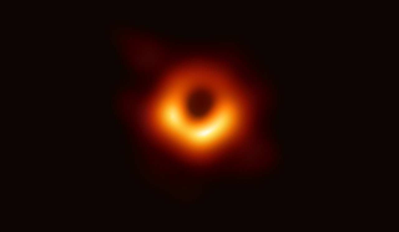
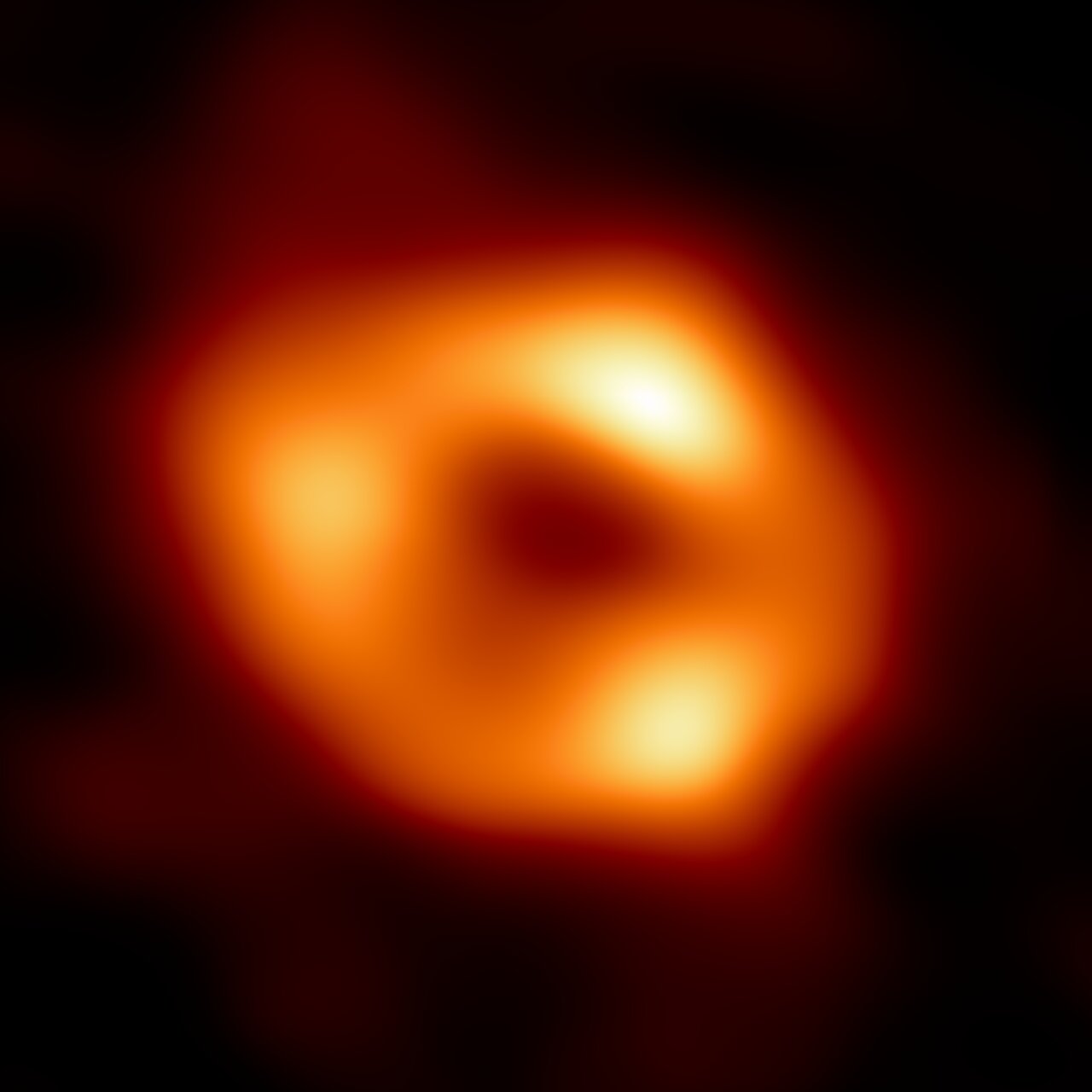
EHT Collaboration / ESO · CC BY 4.0 · eso1907a (M87*, 2019), eso2208-eht-mwa (Sgr A*, 2022)

Open solutions: what we can (and cannot) integrate

Excellent open-source relativistic ray-tracing codes exist, GYOTO (Observatoire de Paris), RAPTOR, ipole, grtrans, Blacklight, and an open implementation of Luminet's method. But they are offline codes (C/C++/Python) computing single frames in minutes/hours: they cannot run in real time inside a WebGL fragment shader in the browser.

What we genuinely integrate are their physical–mathematical formulations: the Schwarzschild geodesic, the Novikov–Thorne disk, the g factor and the Iᵥ/ν³ invariant, the blackbody color. Our shader reimplements them in GLSL and cites them; it does not embed the external code. Stating this is part of the "fail loud, never fake" rule.

Frequently asked questions

References & sources

1. S. M. Carroll, “Lecture Notes on General Relativity”, Schwarzschild geodesics (Caltech).
2. K. Kokkotas, “Particle Trajectories & The Classical Tests”, General Relativity, Universität Tübingen.
3. C. Hirata, “Geodesics in the Schwarzschild geometry”, ph6820, The Ohio State University.
4. J.-P. Luminet (1979), “Image of a spherical black hole with thin accretion disk”, Astronomy & Astrophysics 75, 228.
5. S. E. Gralla, D. E. Holz & R. M. Wald (2019), “Black hole shadows, photon rings, and lensing rings”, Physical Review D 100, 024018.
6. M. D. Johnson et al. (2020), “Universal interferometric signatures of a black hole's photon ring”, Science Advances 6, eaaz1310.
7. N. I. Shakura & R. A. Sunyaev (1973), Astronomy & Astrophysics 24, 337.
8. I. D. Novikov & K. S. Thorne (1973), “Astrophysics of Black Holes”, in Black Holes (Les Houches).
9. D. N. Page & K. S. Thorne (1974), “Disk-accretion onto a black hole. Time-averaged structure of accretion disk”, ApJ 191, 499.
10. B. Paczyński & P. J. Wiita (1980), Astronomy & Astrophysics 88, 23.
11. M. J. Rees (1988), “Tidal disruption of stars by black holes…”, Nature 333, 523.
12. P. C. Peters (1964), “Gravitational radiation and the motion of two point masses”, Physical Review 136, B1224.
13. J. M. Bardeen (1973), “Timelike and null geodesics in the Kerr metric”, in Black Holes (Les Houches).
14. H. Yoshida (1990), “Construction of higher order symplectic integrators”, Physics Letters A 150, 262, the 6th-order symplectic integrator in the Orbits demo.
15. M. Tao (2016), “Explicit symplectic approximation of nonseparable Hamiltonians”, Physical Review E 94, 043303, the method behind the Ultra mode (6th-order symplectic Yoshida for the lensing).
16. L. Flamm (1916), “Beiträge zur Einsteinschen Gravitationstheorie”, Physikalische Zeitschrift 17, 448, the paraboloid.
17. O. James, E. von Tunzelmann, P. Franklin & K. S. Thorne (2015), “Gravitational lensing by spinning black holes… Interstellar”, Classical and Quantum Gravity 32, 065001.
18. F. H. Vincent et al. (2011), “GYOTO: a new general relativistic ray-tracing code”, Classical and Quantum Gravity 28, 225011.
19. C. W. Misner, K. S. Thorne & J. A. Wheeler, “Gravitation” (1973); J. B. Hartle, “Gravity” (2003).
20. Blackbody color → sRGB: N. Bartlett's Planckian-locus approximation (data by M. Charity).
21. Real sky: NASA/Goddard SVS, “Deep Star Maps 2020”, an all-sky equirectangular map from the Gaia/Tycho catalogs (public domain).
22. Real sky (alternative): ESO/S. Brunier, GigaGalaxy Zoom, an all-sky panorama (CC BY 4.0).
23. M. Janssen et al. (2025), “Deep learning inference with the Event Horizon Telescope I–III”, A&A 698, A60–A62: Bayesian neural networks on EHT data. For Sgr A* they point to a near-maximal spin (a ≈ 0.8–0.9, prograde) and a near face-on disk, with emission dominated by hot disk electrons rather than a jet, consistent with the Kerr presets we use.
24. M. Gorski & L. Murchikova (2026), “The Discovery of an Active Wind from the Milky Way's Central Black Hole”, ApJL: first evidence (ALMA + Chandra) of an active wind from Sgr A*, a ~1 pc conical cavity cleared of cold gas. INAF coverage.
25. NASA/Goddard Space Flight Center (2024), “New NASA Black Hole Visualization Takes Viewers Beyond the Brink”: for a 4.3-million-M☉ black hole (Sagittarius A*'s mass), an event horizon of about 25 million km (~17% of the Earth–Sun distance); once crossed, spaghettification arrives 12.8 seconds later, after covering ~128,000 km toward the singularity.
26. INAF (2026), “A nearby black hole to understand the distant past”: SDSS J110546 hosts a relatively low-mass but rapidly growing black hole, with persistent radio emission for over 8 years and a newly formed relativistic jet — a real observational example of the phenomenon this simulation's stylized “Jets” toggle represents.
27. M. Toscani et al. (2025), “Updated predictions for gravitational wave emission from tidal disruption events…”, A&A 703, A75: gravitational waves from tidal disruption events, the phenomenon reproduced in the playground.
28. Stack: Three.js, React Three Fiber, @react-three/drei, @react-three/postprocessing, KaTeX. A native WebGPU renderer (WGSL shader, same physics) also exists at /en/lab/black-hole/webgpu. Development: Fosforonero, Matteo Pizzi (Rome, Italy).